Creating the 2018-2019 math & ELA proficiency map
Antonio R. Vargas
1 Introduction
This note will detail the process I used to create my maps of math and English language arts proficiency in Oregon public schools. These maps show, for each public school in Oregon, the percentage of students who scored at or above the level of “proficient” on the statewide standardized assessments given in the 2018-2019 school year.
1.1 Software packages and options
We will use the R programming language to process the data and create the maps.
To plot the boundary of Oregon, plus roads and bodies of water for orientation, I’ve written a small R package called ormask. You can install it from my github using the following command.
devtools::install_github("szego/ormask")There is around 62 MB of data contained in the ormask package.
In total, these are the packages and options we’ll use:
# data manipulation
library(openxlsx)
library(dplyr)
library(stringr)

# spatial features
library(sf)

# plotting
library(ggplot2)
library(scales)
library(ggvoronoi)
library(ormask)

# options
options(stringsAsFactors = FALSE)

# helper functions

# Calculates the geodesic distance between two points
# specified by radian latitude/longitude using the
# Haversine formula.
# Author: Mario Pineda-Krch
.arcdist <- function(long1, lat1, long2, lat2) {
    long1 <- long1*pi/180  # Convert degrees to radians
    lat1 <- lat1*pi/180
    long2 <- long2*pi/180
    lat2 <- lat2*pi/180
    R <- 6371  # Earth mean radius in km
    delta.long <- (long2 - long1)
    delta.lat <- (lat2 - lat1)
    a <- sin(delta.lat/2)^2 + cos(lat1) * cos(lat2) * sin(delta.long/2)^2
    c <- 2 * asin(min(1,sqrt(a)))
    d = R * c
    return(d)  # Distance in km
}
arcdist <- Vectorize(.arcdist)
2 The data: why, what, and how
Our first goal is to assign longitude and latitude coordinates to the assessment results. It turns out that this necessitates linking several pieces of data from different sources.
The assessment results published by ODE identify schools by school name and district name. There are multiple schools with the same name, but the combination of school name and district name does uniquely identify a school.
ODE includes school numbers and district numbers in its data, but unfortunately these are not the same identification numbers used by the NCES for school locations and geoassignments. And since the NCES school locations data does not contain district names, we will need to add those in order to match the coordinates with the ODE assessment data.
Finally, the assessment results and NCES geoassignments include schools that provide most or all of their instruction virtually. For the purposes of the map, we would like to remove the schools classified as “focus virtual” or “full virtual” from the data.1 ODE’s institution lookup database contains information on virtual status for each school, but this database changes frequently as schools open, close, or otherwise change status. I’ve extracted the focus & full virtual schools as of November 1, 2019 into an excel file hosted on my webpage to ensure that others will be able to replicate the steps of this analysis in the future.
So, the data we need are:
- Coordinates of public schools from NCES
- District information from NCES
- Assessment results from ODE
- The list of schools that are “focus virtual” or “full virtual” from my website
The code below fetches all of this data from the web and saves it in R’s current working directory so that it can be loaded below.
# School coordinates
download.file(
    "https://nces.ed.gov/programs/edge/data/EDGE_GEOCODE_PUBLICSCH_1718.zip",
    "publicsch.zip"
)
unzip("publicsch.zip")
file.remove("publicsch.zip")

# School district coordinates
download.file(
    "https://nces.ed.gov/programs/edge/data/EDGE_GEOCODE_PUBLICLEA_1718.zip",
    "publiclea.zip"
)
unzip("publiclea.zip")
file.remove("publiclea.zip")

# Math assessment results
download.file(
    "https://www.oregon.gov/ode/educator-resources/assessment/Documents/TestResults2019/pagr_schools_math_all_1819.xlsx",
    "pagr_schools_math_all_1819.xlsx",
    mode = "wb"
)

# English language arts assessment results
download.file(
    "https://www.oregon.gov/ode/educator-resources/assessment/Documents/TestResults2019/pagr_schools_ela_all_1819.xlsx",
    "pagr_schools_ela_all_1819.xlsx",
    mode = "wb"
)

# List of focus virtual and full virtual schools
download.file(
    "https://szego.github.io/data/focus_or_full_virtual_2019-11-01.xlsx",
    "focus_or_full_virtual_2019-11-01.xlsx",
    mode = "wb"
)
This downloads about 39 MB worth of data. After extracting the archives, the final size of the files is around 204 MB.
2.1 School coordinates
Here we load the EDGE school and district data.
Each school has a 12-digit identification number called the NCESSCH. The first 7 digits of this code identifies the school district—this number is called the LEAID.2 In the code below we load the school and district data, filter out non-Oregon schools, extract the LEAID from each school’s NCESSCH, and add district names to the school data by matching up the LEAIDs. We also store the coordinate reference system from the EDGE data for later use.
districts <- st_read("EDGE_GEOCODE_PUBLICLEA_1718") %>%
    filter(STATE == "OR") %>%
    as.data.frame() %>%
    select(LEAID, district = NAME)

coordinates <- st_read("EDGE_GEOCODE_PUBLICSCH_1718") %>%
    filter(STATE == "OR") %>%
    mutate(LEAID = NCESSCH %>% str_sub(1, 7)) %>%
    left_join(districts, by = "LEAID") %>%
    select(-LEAID)

schools_crs <- st_crs(coordinates)
Since the EDGE data is for the 2017-2018 school year, we need to update it to match the 2018-2019 assessment data. Careful inspection of the data3 revealed that 10 schools changed their name and 3 schools opened for the first time or reopened after being closed for the 2017-2018 school year. The code below replaces the old school names and adds the three new schools along with their districts and latitude+longitude (obtained from Google Maps).
coordinates <- coordinates %>%
    as.data.frame() %>%
    select(school = NAME, LAT, LON, district) %>%
    mutate(
        school = school %>%
            recode(             # update schools that changed their name
                "REALMS (Rimrock Expeditionary Alternative Learning Middle Sc" =
                    "Realms Middle School",
                "Wood Elementary" = "Powell Butte Elementary School",
                "Buff Intermediate School" = "Buff Elementary School",
                "Madras Primary School" = "Madras Elementary School",
                "McKenzie High School" = "McKenzie River Community School",
                "Multisensory Learning Academy" = "Multnomah Learning Academy",
                "Wellness Business and Sports School" =
                    "Wellness, Business and Sports School",
                "Woodburn Academy of Art Science and Technology" =
                    "Woodburn Academy of Art, Science and Technology",
                "Bridges Career and Technical High School" = "Bridges High School",
                "Falcon Heights Academy" = "Falcon Heights"
            )
    ) %>%
    rbind(data.frame(           # add new schools that opened/reopened
        school = c(
            "Gib Olinger Elementary School",
            "Harriet Tubman Middle School",
            "Rose City Park"
        ),
        district = c(
            "Milton-Freewater Unified SD 7",
            "Portland SD 1J",
            "Portland SD 1J"
        ),
        LAT = c(45.926719, 45.539539, 45.539513),
        LON = c(-118.382083, -122.669166, -122.604070)
    ))
2.2 Assessment results
Now we will load the math and English language arts assessment results. Processing these files is relatively straightforward; we remove virtual schools and schools with missing data, convert the percentages of proficient students to proportions by dividing by 100, and remove some special characters in school names.
The only tricky problem here is how to deal with cases where “< 5.0%” or “> 95.0%” appears in the data instead of the exact proportion of students scoring at or above proficiency. We opt to count these as 5% and 95%, respectively.
virtual <- read.xlsx("focus_or_full_virtual_2019-11-01.xlsx") %>%
    mutate_if(is.character, as.numeric)

math <- read.xlsx("pagr_schools_math_all_1819.xlsx") %>%
    filter(
        Student.Group == "Total Population (All Students)",
        !(School.ID %in% virtual$id)         # remove virtual schools
    ) %>%
    select(
        district = District,
        school = School,
        proficient = `Percent.Proficient.(Level.3.or.4)`
    ) %>%
    mutate(
        proficient = proficient %>%          # replace suppressed or missing entries with NA
            na_if("--") %>%
            na_if("*"),
        proficient = case_when(              # replace intervals with endpoints
            proficient == "< 5.0%" ~ "5",
            proficient == "> 95.0%" ~ "95",
            TRUE ~ proficient
        ) %>%
            as.numeric(),
        proficient = proficient / 100,       # convert percents to proportions
        school = school %>%
            str_replace("\\p{Pd}", "-")      # make all dashes identical
    )

str(math)
## 'data.frame': 1202 obs. of 3 variables:
## $ district : chr "Adel SD 21" "Adrian SD 61" "Adrian SD 61" "Alsea SD 7J" ...
## $ school : chr "Adel Elementary School" "Adrian Elementary School" "Adrian High School" "Alsea Charter School" ...
## $ proficient: num NA 0.436 0.263 0.198 0.448 0.229 0.272 NA 0.369 0.414 ...The procedure for loading the English language arts results is identical to the procedure for the math results.
ela <- read.xlsx("pagr_schools_ela_all_1819.xlsx") %>%
    filter(
        Student.Group == "Total Population (All Students)",
        !(School.ID %in% virtual$id)         # remove virtual schools
    ) %>%
    select(
        district = District,
        school = School,
        proficient = `Percent.Proficient.(Level.3.or.4)`
    ) %>%
    mutate(
        proficient = proficient %>%          # replace suppressed or missing entries with NA
            na_if("--") %>%
            na_if("*"),
        proficient = case_when(              # replace intervals with endpoints
            proficient == "< 5.0%" ~ "5",
            proficient == "> 95.0%" ~ "95",
            TRUE ~ proficient
        ) %>%
            as.numeric(),
        proficient = proficient / 100,       # convert percents to proportions
        school = school %>%
            str_replace("\\p{Pd}", "-")      # make all dashes identical
    )

str(ela)
## 'data.frame': 1202 obs. of 3 variables:
## $ district : chr "Adel SD 21" "Adrian SD 61" "Adrian SD 61" "Alsea SD 7J" ...
## $ school : chr "Adel Elementary School" "Adrian Elementary School" "Adrian High School" "Alsea Charter School" ...
## $ proficient: num NA 0.644 0.632 0.263 0.476 0.592 0.476 0.4 0.385 0.58 ...2.3 Associating assessment results with coordinates
The last thing we need to do is assign coordinates to the assessment results. In most cases this is simple, but we need to decide how to handle different schools with the same coordinates. Apparently these schools share a single building or campus. To further complicate things, there are schools who share the same building but have slightly different coordinates in the data.
Careful inspection of the data indicates that schools whose coordinates are within 30 meters of each other share the same building, and that there are nearby but distinct school buildings more than 30 meters apart. As such, we will assign all schools within 30 meters of another school the same coordinates. This is an imperfect cutoff but it seems appropriate given the limitations of the data.
The code below does the coordinate combining.
already_adjusted <- c()

for(i in 1:nrow(coordinates))  # loop through each school in the data
    if(!(i %in% already_adjusted)) {
        near_i <- which(  # find schools within 30 meters of the current school
            arcdist(
                coordinates$LON[i],
                coordinates$LAT[i],
                coordinates$LON,
                coordinates$LAT
            ) < 0.03  # km
        )

        # assign nearby schools the same longitude and latitude
        coordinates$LON[near_i] <- coordinates$LON[i]
        coordinates$LAT[near_i] <- coordinates$LAT[i]

        # exclude nearby schools from future iterations
        already_adjusted <- c(already_adjusted, near_i)
    }
Once the coordinates have been combined, we can join the assessment results to the coordinates using the school and district names as identifiers.
To represent the proficiency percentage for a building containing multiple schools we use the average of the proficiency percentages of the individual schools. This is not an ideal solution to the problem. It would be preferable to weight the percentages according to the numbers of assessment participants in each school, but these counts are suppressed by ODE when more than 95% or fewer than 5% of the participants at a school score at or above proficiency on the assessment.
The code below carries out these steps and does some extra work to convert the resulting data into spatial feature objects.
coordinates_math <- coordinates %>%
    inner_join(math, by = c("school", "district")) %>%
    group_by(LAT, LON) %>%  # combine schools in the same building
    summarize(
        proficient = if_else(
            sum(is.na(proficient)) == length(proficient),
            NA_real_,
            mean(proficient, na.rm = TRUE)  # take the average of the proficient percents
        )                                   # of the schools in the same building
    ) %>%
    ungroup() %>%
    mutate(  # add a spatial feature column of longitude and latitude coordinates
        geometry = st_sfc(
            lapply( 1:n(), function(i) st_point(c(LON[i], LAT[i])) ),
            crs = st_crs(schools_crs)
        )
    ) %>%
    st_sf()  # convert to a spatial feature object

coordinates_ela <- coordinates %>%
    inner_join(ela, by = c("school", "district")) %>%
    group_by(LAT, LON) %>%  # combine schools in the same building
    summarize(
        proficient = if_else(
            sum(is.na(proficient)) == length(proficient),
            NA_real_,
            mean(proficient, na.rm = TRUE)  # take the average of the proficient percents
        )                                   # of the schools in the same building
    ) %>%
    ungroup() %>%
    mutate(  # add a spatial feature column of longitude and latitude coordinates
        geometry = st_sfc(
            lapply( 1:n(), function(i) st_point(c(LON[i], LAT[i])) ),
            crs = st_crs(schools_crs)
        )
    ) %>%
    st_sf()  # convert to a spatial feature object
This concludes the data processing part of the project.
3 Creating the maps
Once we’ve created a spatial feature object containing longitude, latitude, and proportions of students scoring at or above proficiency, making the maps is relatively straightforward using ggplot2 and the ggvoronoi package.
We create the Voronoi diagram, apply a mask to cover up the area surrounding Oregon, tweak the color scheme4 and legend, and remove some unnecessary elements of the plot.
The mask around oregon is inserted by the oregon_mask() function from the ormask package.5
gg_math <- ggplot() +
    geom_voronoi(
        aes(x = LON, y = LAT, fill = proficient),
        data = coordinates_math
    ) +
    oregon_mask() +  # from the ormask package
    scale_fill_viridis_c(
        name = "% of students\nat or above\nproficiency",
        breaks = (0:5)/5,
        labels = percent_format(accuracy = 1),
        option = "plasma"  # try "viridis", "magma", or "plasma"
    ) +
    ggtitle("Oregon Math Assessment Proficiency 2018-19") +
    theme(
        axis.title.x = element_blank(),
        axis.text.x = element_blank(),
        axis.ticks.x = element_blank(),
        axis.title.y = element_blank(),
        axis.text.y = element_blank(),
        axis.ticks.y = element_blank()
    )

gg_math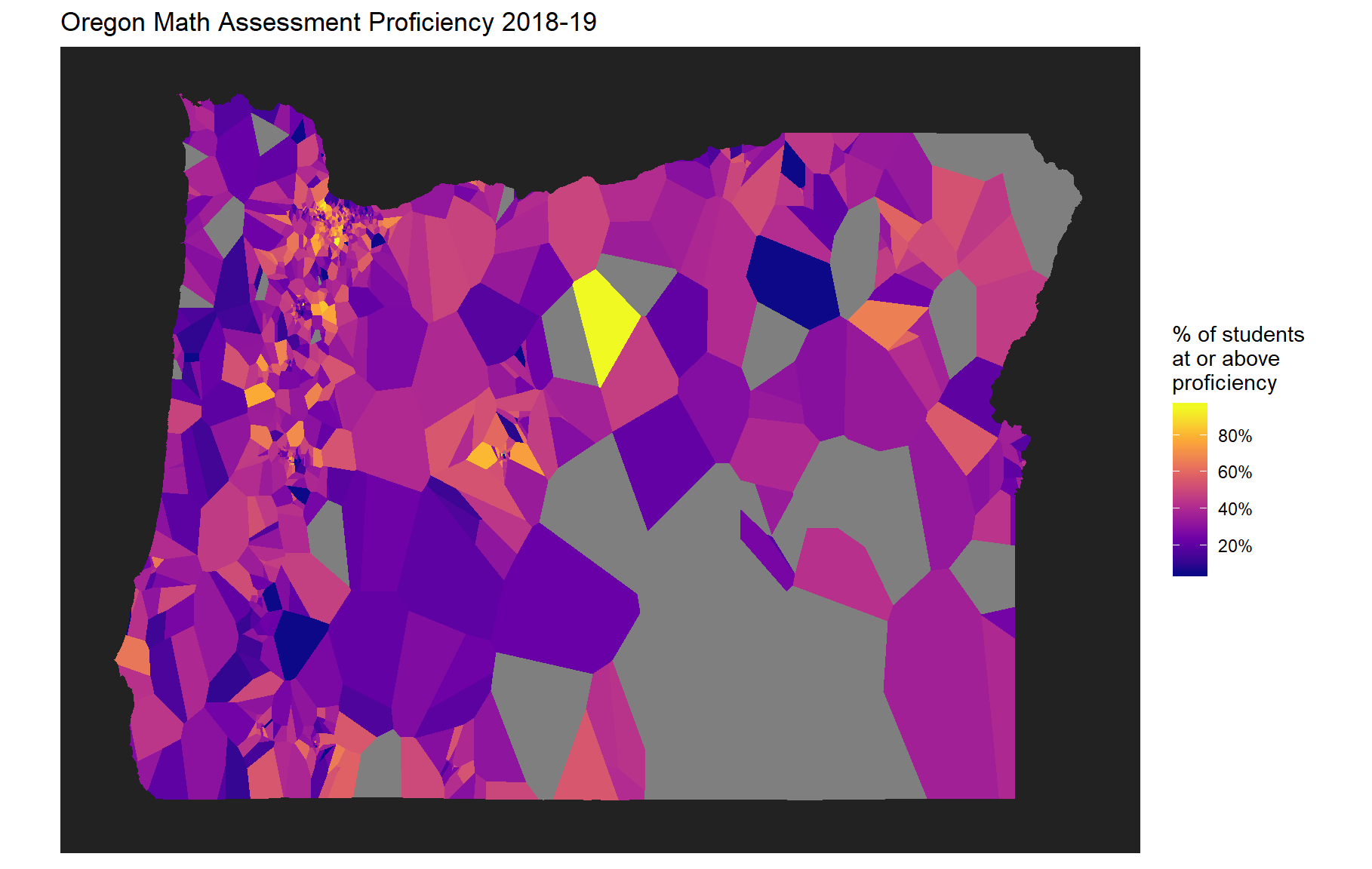
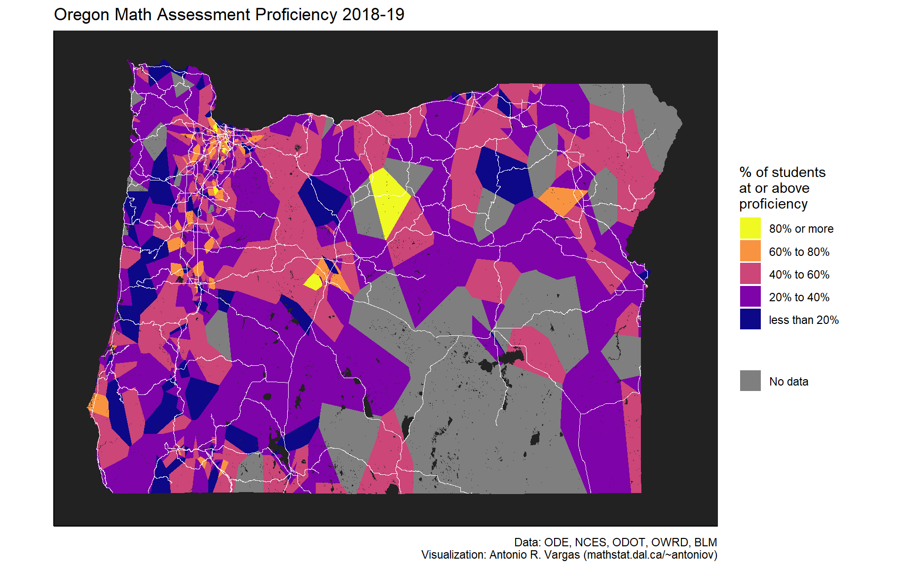
The final maps used a discrete color scale rather than a continuous one as in the maps above. The way I ended up doing this was a bit ad hoc, so rather than trying to explain the details I’ll just present the code which achieves the desired effect.
Do note that the final map below includes major roads and bodies of water.6 These features of ormask are intended to help the viewer orient themselves within the state when viewing the maps in full resolution.7 Be warned that the water does take a long time to render due to the amount of fine detail.
levels <- c(
    "less than 20%",
    "20% to 40%",
    "40% to 60%",
    "60% to 80%",
    "80% or more"
)

coordinates_math %>%
    mutate(
        proficient = case_when(
            is.na(proficient) ~ NA_character_,
            proficient < 0.2 ~ levels[1],
            proficient < 0.4 ~ levels[2],
            proficient < 0.6 ~ levels[3],
            proficient < 0.8 ~ levels[4],
            TRUE ~ levels[5]
        ) %>%
            factor(levels = levels)
    ) %>%
    ggplot() +
    geom_voronoi(
        aes(x = LON, y = LAT, fill = proficient, color = "No data")
    ) +
    oregon_mask(road_color = "white", water_color = "#222222") +  # slow to render
    scale_fill_viridis_d(
        name = "% of students\nat or above\nproficiency",
        option = "plasma",  # try "viridis", "magma", or "plasma"
        guide = guide_legend(order = 1, reverse = TRUE),
        na.translate = FALSE,
        na.value = "grey50"
    ) +
    scale_color_manual(values = NA) +
    guides(
        color = guide_legend(
            title = element_blank(),
            override.aes = list(fill = "grey50")
        )
    ) +
    ggtitle("Oregon Math Assessment Proficiency 2018-19") +
    labs(
        caption = paste(
            "Data: ODE, NCES, ODOT, OWRD, BLM",
            "Visualization: Antonio R. Vargas (szego.github.io)",
            sep = "\n"
        )
    ) +
    theme_classic() +
    theme(
        axis.title.x = element_blank(),
        axis.text.x = element_blank(),
        axis.ticks.x = element_blank(),
        axis.title.y = element_blank(),
        axis.text.y = element_blank(),
        axis.ticks.y = element_blank(),
        panel.background = element_rect(fill = "grey50")
    )
Similar code was used to make the English language arts maps.
If we’re happy with the way our map looks we could save it with a call to ggplot2::ggsave() like the one below.
ggsave(
    "math_proficiency.png",
    gg_math,
    scale = 0.6,
    width = 13,
    height = 9,
    dpi = 1600,  # using a dpi of around 1600 here will give good zoomability
    type = "cairo-png"
)
4 Acknowledgements
I would like to thank Amelia L. Vargas for her integral contributions, including providing insight into and references for Oregon’s virtual schools, explaining relationships between the ODE and NCES datasets, and suggesting the school At-A-Glance Profiles as a means to discover school name changes. Every conversation we had made this project better.
8 December 2019
The different types of virtual schools are explained in ODE’s Virtual School Status FAQ (pdf). See also the 2016 Data Brief on Virtual School Enrollment and Population (pdf) for some insight into student demographics and outcomes in virtual schools.↩
See the EDGE Geocodes Documentation (pdf) for details on the LEAID and NCESSCH identifiers.↩
Searching for a school’s At-A-Glance Profile can reveal the school’s past names. For example, the search result for “Powell Butte Elementary School” indicates that it was previously called “Wood Elementary”. It is called “Wood Elementary” in the EDGE data and “Powell Butte Elementary School” in the assessment data.↩
The colors are from the “plasma” color palette created by Stéfan van der Walt and Nathaniel Smith specifically with people with different forms of colorblindness in mind. For further information see this neat article with examples and this informative talk by the creators explaining some of the color theory.↩
The Oregon mask is derived from the 2001 Oregon State Boundary shapefile from the Oregon office of the BLM.↩
The road data comes from ODOT and the water data from the OWRD. See the documentation of the ormask package for more details.↩
I use the shape of the Willamette River and the bridge over it to locate Salem in the maps and to distinguish Salem from West Salem in the full resolution maps.↩